home /
academic notes /
Identifying QPOs in lightcurve data
A quick and dirty guide for identifying quasi-periodic oscillations (QPOs) in astronomical lightcurve data based on work from the Advanced Data Analysis course at the University of St Andrews.
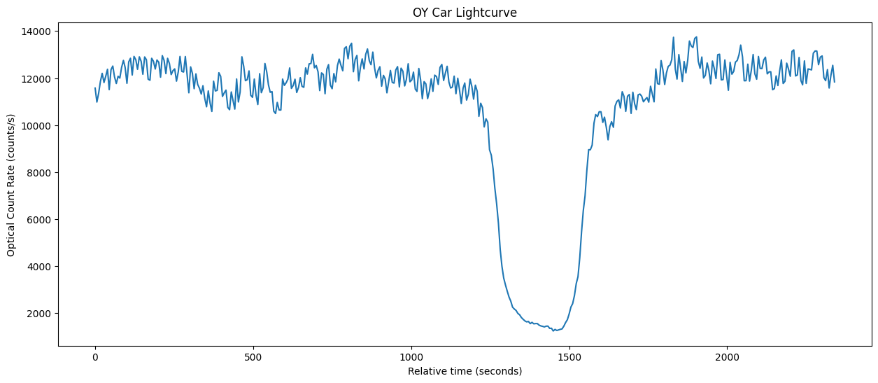
Plotting the raw data
To begin your analysis you'll need three arrays: photon count, uncertainty in photon count, and time relative to start of observation. If your source data exists in the form of a plaintext file, use the numpy loadtxt function with the optional skiprows argument to ignore anything that isn't raw data. I used the following code:
        lightcurve_data = np.loadtxt('your_data.dat', skiprows=15)


        parameter = lightcurve_data[:,i]
Where i is the column number for whatever parameter you're loading.
Now you're going to want to plot the lightcurve to get an understanding of the overall shape. The Matplotlib library is a standard in the sciences, but any plotting library will work fine.
Smoothing the lightcurve
If the length of your observation significantly exceeds the period of the QPOs you're looking for, your lightcurve may have an underlying shape which you'll want to remove before your analysis. To do this we're going to create a smooth function loosely based on the lightcurve. You want this function to fit the overall shape of the lightcurve but not the short-scale variations. The two best strategies are to use a spline function or a running optimal average (ROA) with a Gaussian memory function.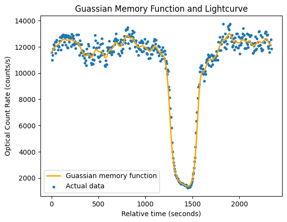
For a spline function, use the SciPy splrep and BSpline functions as follows:
        tck = splrep(time_array, count_array, w=1/uncertainty_array**2, s=0.9)


        smoothed_array = BSpline(*tck)(time_array)
For the splrep function, s is a parameter which controls the looseness of
the fit. Experiment with different values and plot them until your
smoothing function fits the criteria above.
Alternatively, use a ROA with a Gaussian memory function as follows: $$\hat X(t) = \frac{\Sigma X_i w_i(t)}{\Sigma w_i(t)}$$ $$w_i(t) = \frac{G(t-t_i)}{\sigma_i(t)^2}$$ Where \( X_i \) is the i-th element of the photon count array; \(\sigma_i\), the i-th element of the uncertainty array; and \(G(t-t_i)\) the Gaussian function: $$G(t-t_i) = \exp{ \left [-\frac12 \left (\frac{t-t_i}{\tau} \right)^2 \right]}$$ Subtracting this smooth line from your astronomical data will give you a residuals array. This is the data that you're going to analyse your QPOs from.
Fitting to a function
The next step is to try to fit your data to a function. Your best bet is to use something of the form: $$F(t) = B + C\cos (f\;t_i) + S \sin (f\;t_i)$$ which will account for any background noise and let you test your fit for any trial frequency \(f\). The plan is to calculate the maximum likelihood values for the \(B\), \(C\), and \(S\) coefficients and the corresponding \(\chi^2\) value for each trial frequency. This is proportional to the "badness-of-fit" value - AKA a minimum in this value corresponds to a pretty good frequency fit!You're going to need a range of frequency values to test over, so you might as well read up on Nyquist sampling. If you're in a hurry, use the following code:
        N = len(time_array)


        delta_freq = 2 * np.pi / time_array[-1]


        nyq_freq = N*delta_freq/2


        freq_array = np.linspace(delta_freq, nyq_freq+delta_freq, N)
The resulting freq_array is your range of trial frequencies.
MLE parameters and chi squared values
To determine the best-fit coefficients you first need to create an array for each which contains their "pattern". For a constant like \(B\) that array is constructed using np.ones_like(time_array). For the sinusoidal patterns, you'll need to compute the value of \(\cos \; \text{or} \; \sin \left (f \; t_i\right )\) for every value of \(t_i\)Create a pattern matrix \(P\) using the np.vstack function on your three pattern arrays. Next you'll need to create an NxN matrix with inverse data variances \(1/\sigma^2_i\) on the diagonals - call this \(S\).
Create your Hessian matrix according to: $$H = (P \cdot S)\cdot P^T$$ Now construct a correlation vector, \(C\), using your residuals array, \(y\)according to: $$C = (y \cdot S) \cdot P^T$$ Your best-fit coefficients can now be determined using the numpy linalg.solve function:
coefficients = np.linalg.solve(H, C)
The amplitude of this particular sinusoidal function can be found using the formula: $$A = \sqrt{C^2 + S^2}$$ To get a \(\chi^2\) value for this fit, compute the residuals as follows.
        model = P.T @ coefficients


        res = (residuals_array - model)/uncertainty_array


        chi_squared = res @ res
Now just plot \(\chi^2\) against the trial frequencies and look for minima! You should end up with something like this:
Estimating QPO period
To estimate the period of the strongest QPO (or whichever one you want to analyse), you're going to fit a polynomial to the three lowest points of the \(\chi^2\) minimum after converting the frequency array to a period array.p1, p2, and p3 refer to the frequency value of the three lowest points, where b is the lowest, and c1, c2, and c3 refer to the \(\chi^2\) value of the three lowest points.
        # returns the array index for your chi_squared minimum

        min_index = np.where(chi_squared == np.min(chi_squared))[0][0]


        def Quadratic(x, a, b, c):

          return a*x**2 + b*x + c


        def Polynomial(x1, x2, x3, y1, y2, y3):

             a, b, c = curve_fit(Quadratic, [x1, x2, x3] ,[y1, y2, y3])[0]

             xhat = -b/(2*a)

             yhat = Quadratic(xhat, a, b, c)

             sigx = np.sqrt(1/np.abs(a))

             return xhat, yhat, sigx


        p_hat, chiphat, sig_p = Polynomial(p1, p2, p3, c1, c2, c3)
The period and corresponding uncertainty are p_hat and sig_p respectively.
Closing remarks
Congratulations! You've successfully identified a quasi-period oscillation and determined both its period and amplitude. If you want some ideas for next steps, try:- calculating the variation in period and amplitude over time using a memory function
- identify which \(\chi^2\) stalactites are genuine QPOs and which are simply aliasing effects or harmonics