Gravitational Microlensing Primer
When a massive object passes near the line of sight between an observer and background star, its gravitational field will temporarily deflect more light towards the observer, producing an increase in brightness. This is the basic principle of gravitational lensing. We observe this effect by monitoring millions of stars with large survey telescopes, waiting for a chance alignment. If we're lucky, these events may reveal information about planets orbiting the lensing star.
Contents
- Single lens model- Caustics and planet detection
Single lens model
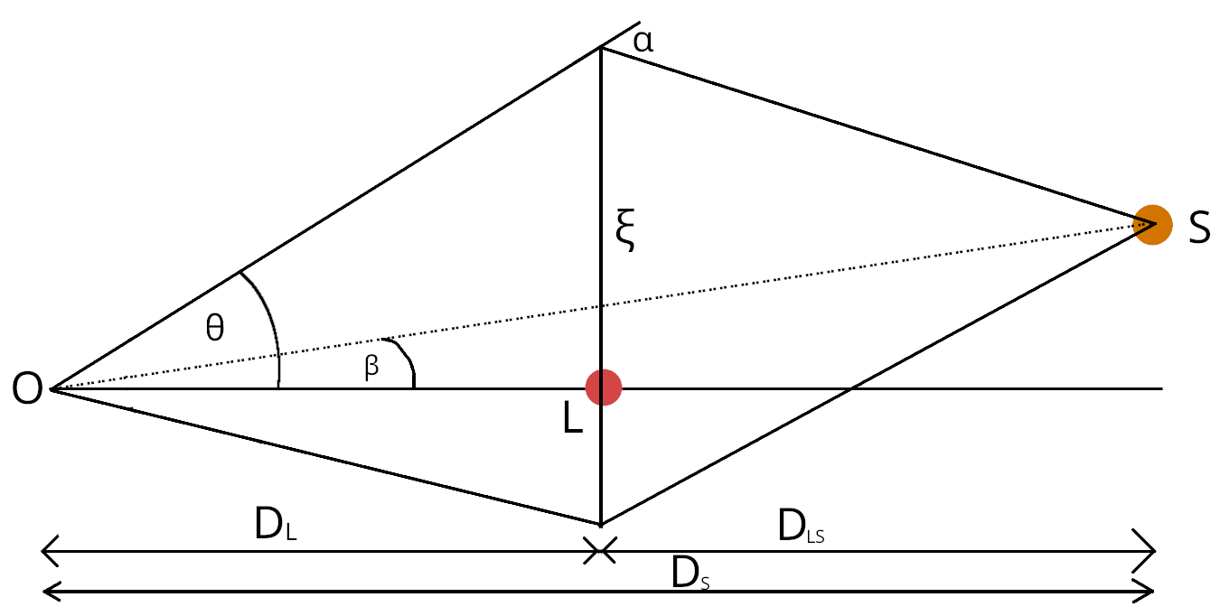
In figure one we illustrate the geometry of a single lens microlensing event. O, L, S refer to the observer, lens
star, source star respectively, \(D_L\) and \(D_S\), the distances to the lens and source stars, and \(D_{LS}\)
the distance between the lens and source stars. \(\beta\) the angular impact parameter of the source, \(\xi\) the
image position of the source star on the lens plane, and \(\alpha\) the angular deflection of the light from the
source.
Geometrically, we can show that the equation relating the image to true source positions is,
\begin{equation}
\beta = \theta - \frac{4GM_L}{c^2 \theta}\frac{D_s-D_L}{D_LD_S}
\end{equation}
From this equation we can define a characteristic scale for microlensing events: the Einstein radius. This is the
degree to which the image of the source would be deflected in the case that observer, lens, and source were
perfectly aligned,
\begin{equation}
\theta_E = \sqrt{\frac{4GM_L}{c^2} \frac{D_S - D_L}{D_LD_S}}
\end{equation}
\begin{equation}
\approx 0.55\;\text{mas}\sqrt{\frac{1-D_L/D_S}{D_L/D_S}} \left ( \frac{D_S}{8kpc}\right)^{-1/2} \left (
\frac{M}{0.3M_{\odot}}\right )^{1/2}
\end{equation}
where \(M_L\) is the sum of the lens system masses. Therefore a typical microlensing event involving a source star
in the galactic bulge and a lens star at half the source distance will have an angular Einstein radius of less
than one milliarcsecond [ Mao, 2008 ]. These scales typically cannot
be
resolved by common telescopes.
If we note that the second term under the square root of equation two is the difference in annual parallax, we can
also define the Einstein radius as,
\begin{equation}
\theta_E = \sqrt{\frac{4GM_L}{c^2}\pi_E}
\end{equation}
which implies that a parallax measurement for the microlensing event can constrain the lens mass parameter
[ Sajadian, 2014 ].
As shown by S. Gaudi [ Gaudi, 2012 ], we can
normalise the impact parameter
\(\beta\) and image deflection \(\theta\) by the Einstein radius and define two coordinates \(u =
\beta/\theta_E\), \(y = \theta / \theta_E\) such that the single lens equation simplifies to,
\begin{equation}
u = y - y^{-1}
\end{equation}
which has two solutions in \(y\),
\begin{equation}
y_{\pm} = \pm \frac12 \left [\sqrt{u^2 + 4} \pm u \right]
\end{equation}
Under Liouville's theorem surface brightness must be conserved in microlensing, and so the magnification at any
point in time is equal to the ratio of sum of the image areas to the source area
[ Batista, 2018 ].
Therefore, taking the inverse of the Jacobian determinant, \(\text{det} \; J\), for this lens equation evaluated
at both image positions gives us the total magnification of the event,
\begin{equation}
A(u) = \frac{u^2 + 2}{u\sqrt{u^2 + 4}}
\end{equation}
\begin{equation}
u(t) = \sqrt{\frac{(t-t_0)^2}{t_E^2} + u_0^2}
\end{equation}
where \(t_E = \theta_E / \mu\) is the Einstein ring crossing time of the event and \(\mu\) the proper relative
motion between lens and source. Assuming that \(\mu\) is uniform and rectilinear, the magnification of a point
lens model can therefore be described entirely by the three parameters \(\{t_E, t_0, u_0\}\)
[ Liebig, 2015 ]. For a typical microlensing observation of a
bulge star, we would expect
an impact parameter in the vicinity of \(0.3-0.5\theta_E\) and an Einstein crossing time of \(t_E \approx 20-30\)
days [ Gaudi, 2000 ].
Caustics and planet detection
For the single lens model, there is only one possible source position in the lens plane that would result in
infinite magnification: directly behind the lens star. This is known as the caustic point of the single lens model. For a lens system
with a secondary object, such as a planet or a binary star, the lens equation becomes a complex fifth-order
polynomial [Han, 2005]. We now also require four more parameters: \(q\), the mass ratio of the primary and
secondary bodies, \(s\), the separation of the two bodies in terms of \(\theta_E\), \(\alpha\), the planet-star
angle, and \(\rho\), the source size relative to \(\theta_E\) [
Liebig, 2015 ]. Solving
for the source positions that would result in \(\text{det} \; J = 0\) as in the single lens case results in a set
of closed curve caustics of finite size, and it is through these caustics that we may detect planets in the lens
system.
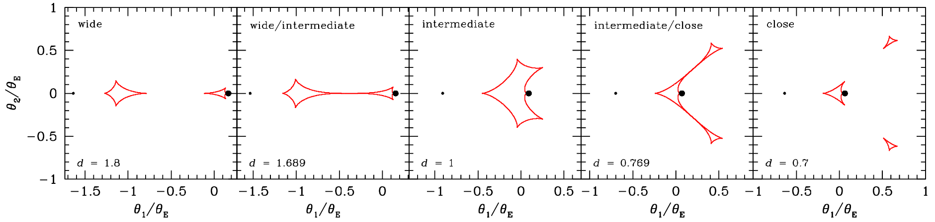
There are three families of caustic morphology in the double lens model that arise as through three distinct
planetary topologies: the close, intermediate, and wide separations. A close topology refers to a system in which
the orbital radius of the planet is less than the Einstein radius of the lens system. In this case there are three
distinct caustics, one central caustic located around the lens star, and two smaller planetary caustics positioned
outside the Einstein ring on the opposite side from the planet. An intermediate topology corresponds to a planet
situated near the Einstein radius, and results in a single, large caustic centred between the primary and
secondary. The wide topology is observed when the secondary lies beyond the Einstein radius. As with the close
topology we have a central caustic located near the primary, but the difference is that the planetary caustic is a
single closed curve situated near the secondary [
Giannini, 2013 ]. These
caustic topologies are illustrated in figure two.
If these caustic regions intersect with the source star, the effect is to perturb the overall light curve in a way that can reveal detailed information on the planetary system. These perturbations persist for a timescale proportional to \(t \sim \sqrt{q}/t_E\), which for an Earth-mass planet may correspond to less than a day [Gould 2005].
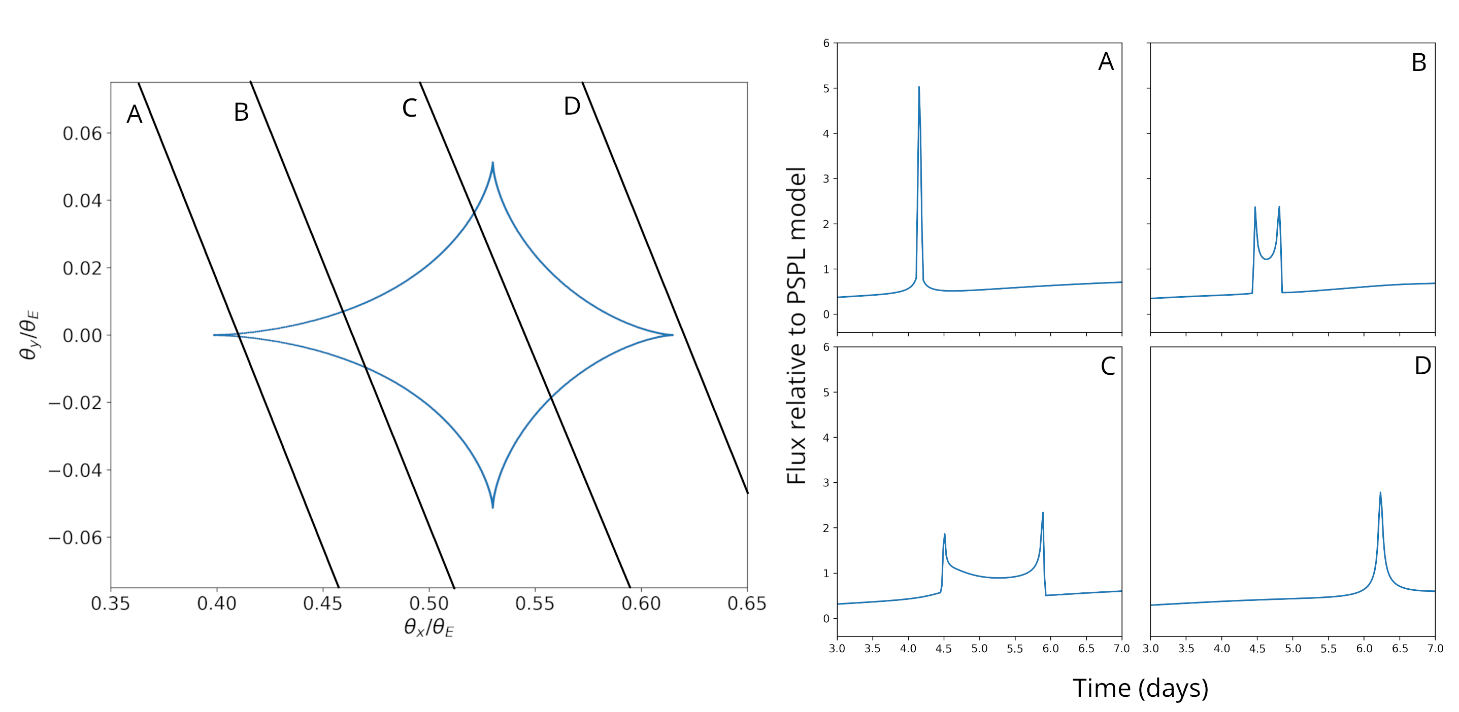
The light curve morphologies of planetary deviations are often degenerate in the sense that different planetary parameters may result in similar signals [ Rahvar, 2015 ]. One example is the degeneracy between central caustics for \(s \leftrightarrow 1/s\) orbital radii, which is more pronounced for lower mass planets [ Chung, 2011 ]. However, careful analysis of perturbation morphologies can allow us to estimate the parameters of orbital radius, mass ratio, and planet-star angle [ Gaudi, 2012 ]. In figure three we presents perturbation residuals for different source paths through the wide topology planetary caustic of an object roughly three times the mass of Jupiter.